9. Orthogonal Projections and Their Applications #

Contents

Orthogonal Projections and Their Applications

9.1. Overview #

Orthogonal projection is a cornerstone of vector space methods, with many diverse applications.

These include

Least squares projection, also known as linear regression
Conditional expectations for multivariate normal (Gaussian) distributions
Gram–Schmidt orthogonalization
QR decomposition
Orthogonal polynomials
etc

In this lecture, we focus on

key ideas
least squares regression

We’ll require the following imports:

import numpy as np
from scipy.linalg import qr

9.1.1. Further Reading#

For background and foundational concepts, see our lecture on linear algebra.

For more proofs and greater theoretical detail, see A Primer in Econometric Theory.

For a complete set of proofs in a general setting, see, for example, [Roman, 2005].

For an advanced treatment of projection in the context of least squares prediction, see this book chapter.

9.2. Key Definitions #

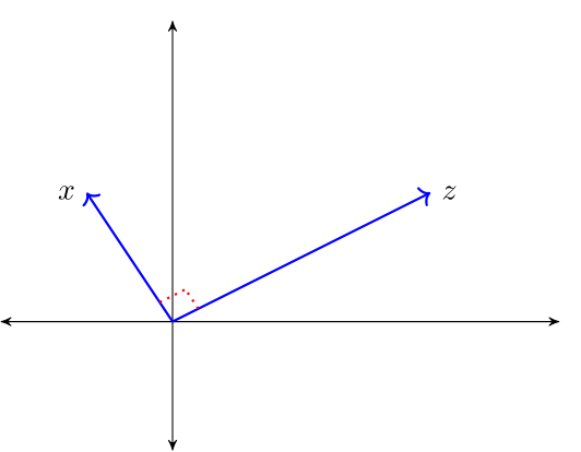
Assume $x, z \in R^{n}$ .

Define $⟨ x, z ⟩ = \sum_{i} x_{i} z_{i}$ .

Recall $‖ x ‖^{2} = ⟨ x, x ⟩$ .

The law of cosines states that $⟨ x, z ⟩ = ‖ x ‖ ‖ z ‖ \cos (θ)$ where $θ$ is the angle between the vectors $x$ and $z$ .

When $⟨ x, z ⟩ = 0$ , then $\cos (θ) = 0$ and $x$ and $z$ are said to be orthogonal and we write $x ⊥ z$ .

For a linear subspace $S \subset R^{n}$ , we call $x \in R^{n}$ orthogonal to $S$ if $x ⊥ z$ for all $z \in S$ , and write $x ⊥ S$ .

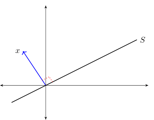
The orthogonal complement of linear subspace $S \subset R^{n}$ is the set $S^{⊥} := {x \in R^{n} : x ⊥ S}$ .

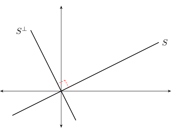
$S^{⊥}$ is a linear subspace of $R^{n}$

To see this, fix $x, y \in S^{⊥}$ and $α, β \in R$ .
Observe that if $z \in S$ , then

⟨ α x + β y, z ⟩ = α ⟨ x, z ⟩ + β ⟨ y, z ⟩ = α \times 0 + β \times 0 = 0

Hence $α x + β y \in S^{⊥}$ , as was to be shown

A set of vectors ${x_{1}, \dots, x_{k}} \subset R^{n}$ is called an orthogonal set if $x_{i} ⊥ x_{j}$ whenever $i \neq j$ .

If ${x_{1}, \dots, x_{k}}$ is an orthogonal set, then the Pythagorean Law states that

‖ x_{1} + \dots + x_{k} ‖^{2} = ‖ x_{1} ‖^{2} + \dots + ‖ x_{k} ‖^{2}

For example, when $k = 2$ , $x_{1} ⊥ x_{2}$ implies

‖ x_{1} + x_{2} ‖^{2} = ⟨ x_{1} + x_{2}, x_{1} + x_{2} ⟩ = ⟨ x_{1}, x_{1} ⟩ + 2 ⟨ x_{2}, x_{1} ⟩ + ⟨ x_{2}, x_{2} ⟩ = ‖ x_{1} ‖^{2} + ‖ x_{2} ‖^{2}

9.2.1. Linear Independence vs Orthogonality#

If $X \subset R^{n}$ is an orthogonal set and $0 \notin X$ , then $X$ is linearly independent.

Proving this is a nice exercise.

While the converse is not true, a kind of partial converse holds, as we’ll see below.

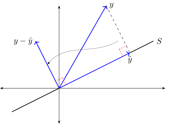
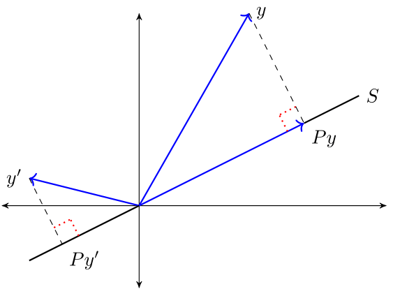
9.3. The Orthogonal Projection Theorem #

What vector within a linear subspace of $R^{n}$ best approximates a given vector in $R^{n}$ ?

The next theorem answers this question.

Theorem (OPT) Given $y \in R^{n}$ and linear subspace $S \subset R^{n}$ , there exists a unique solution to the minimization problem

\hat{y} := a r g m i n_{z \in S} ‖ y - z ‖

The minimizer $\hat{y}$ is the unique vector in $R^{n}$ that satisfies

$\hat{y} \in S$
$y - \hat{y} ⊥ S$

The vector $\hat{y}$ is called the orthogonal projection of $y$ onto $S$ .

The next figure provides some intuition

9.3.1. Proof of Sufficiency#

We’ll omit the full proof.

But we will prove sufficiency of the asserted conditions.

To this end, let $y \in R^{n}$ and let $S$ be a linear subspace of $R^{n}$ .

Let $\hat{y}$ be a vector in $R^{n}$ such that $\hat{y} \in S$ and $y - \hat{y} ⊥ S$ .

Let $z$ be any other point in $S$ and use the fact that $S$ is a linear subspace to deduce

‖ y - z ‖^{2} = ‖ (y - \hat{y}) + (\hat{y} - z) ‖^{2} = ‖ y - \hat{y} ‖^{2} + ‖ \hat{y} - z ‖^{2}

Hence $‖ y - z ‖ \geq ‖ y - \hat{y} ‖$ , which completes the proof.

9.3.2. Orthogonal Projection as a Mapping#

For a linear space $Y$ and a fixed linear subspace $S$ , we have a functional relationship

y \in Y \mapsto its orthogonal projection \hat{y} \in S

By the OPT, this is a well-defined mapping or operator from $R^{n}$ to $R^{n}$ .

In what follows we denote this operator by a matrix $P$

$P y$ represents the projection $\hat{y}$ .
This is sometimes expressed as ${\hat{E}}_{S} y = P y$ , where $\hat{E}$ denotes a wide-sense expectations operator and the subscript $S$ indicates that we are projecting $y$ onto the linear subspace $S$ .

The operator $P$ is called the orthogonal projection mapping onto $S$ .

It is immediate from the OPT that for any $y \in R^{n}$

$P y \in S$ and
$y - P y ⊥ S$

From this, we can deduce additional useful properties, such as

$‖ y ‖^{2} = ‖ P y ‖^{2} + ‖ y - P y ‖^{2}$ and
$‖ P y ‖ \leq ‖ y ‖$

For example, to prove 1, observe that $y = P y + y - P y$ and apply the Pythagorean law.

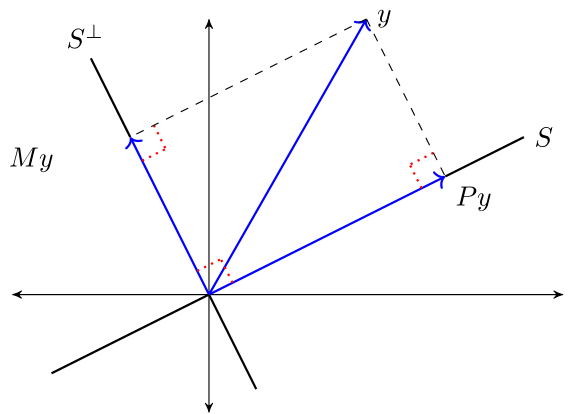
9.3.2.1. Orthogonal Complement#

Let $S \subset R^{n}$ .

The orthogonal complement of $S$ is the linear subspace $S^{⊥}$ that satisfies $x_{1} ⊥ x_{2}$ for every $x_{1} \in S$ and $x_{2} \in S^{⊥}$ .

Let $Y$ be a linear space with linear subspace $S$ and its orthogonal complement $S^{⊥}$ .

We write

Y = S \oplus S^{⊥}

to indicate that for every $y \in Y$ there is unique $x_{1} \in S$ and a unique $x_{2} \in S^{⊥}$ such that $y = x_{1} + x_{2}$ .

Moreover, $x_{1} = {\hat{E}}_{S} y$ and $x_{2} = y - {\hat{E}}_{S} y$ .

This amounts to another version of the OPT:

Theorem. If $S$ is a linear subspace of $R^{n}$ , ${\hat{E}}_{S} y = P y$ and ${\hat{E}}_{S^{⊥}} y = M y$ , then

P y ⊥ M y and y = P y + M y for all y \in R^{n}

The next figure illustrates

9.4. Orthonormal Basis #

An orthogonal set of vectors $O \subset R^{n}$ is called an orthonormal set if $‖ u ‖ = 1$ for all $u \in O$ .

Let $S$ be a linear subspace of $R^{n}$ and let $O \subset S$ .

If $O$ is orthonormal and $span O = S$ , then $O$ is called an orthonormal basis of $S$ .

$O$ is necessarily a basis of $S$ (being independent by orthogonality and the fact that no element is the zero vector).

One example of an orthonormal set is the canonical basis ${e_{1}, \dots, e_{n}}$ that forms an orthonormal basis of $R^{n}$ , where $e_{i}$ is the $i$ th unit vector.

If ${u_{1}, \dots, u_{k}}$ is an orthonormal basis of linear subspace $S$ , then

x = \sum_{i = 1}^{k} ⟨ x, u_{i} ⟩ u_{i} for all x \in S

To see this, observe that since $x \in span {u_{1}, \dots, u_{k}}$ , we can find scalars $α_{1}, \dots, α_{k}$ that verify

(9.1)#

x = \sum_{j = 1}^{k} α_{j} u_{j}

Taking the inner product with respect to $u_{i}$ gives

⟨ x, u_{i} ⟩ = \sum_{j = 1}^{k} α_{j} ⟨ u_{j}, u_{i} ⟩ = α_{i}

Combining this result with (9.1) verifies the claim.

9.4.1. Projection onto an Orthonormal Basis#

When a subspace onto which we project is orthonormal, computing the projection simplifies:

Theorem If ${u_{1}, \dots, u_{k}}$ is an orthonormal basis for $S$ , then

(9.2)#

P y = \sum_{i = 1}^{k} ⟨ y, u_{i} ⟩ u_{i}, \forall y \in R^{n}

Proof: Fix $y \in R^{n}$ and let $P y$ be defined as in (9.2).

Clearly, $P y \in S$ .

We claim that $y - P y ⊥ S$ also holds.

It sufficies to show that $y - P y ⊥$ any basis vector $u_{i}$ .

This is true because

⟨ y - \sum_{i = 1}^{k} ⟨ y, u_{i} ⟩ u_{i}, u_{j} ⟩ = ⟨ y, u_{j} ⟩ - \sum_{i = 1}^{k} ⟨ y, u_{i} ⟩ ⟨ u_{i}, u_{j} ⟩ = 0

(Why is this sufficient to establish the claim that $y - P y ⊥ S$ ?)

9.5. Projection Via Matrix Algebra #

Let $S$ be a linear subspace of $R^{n}$ and let $y \in R^{n}$ .

We want to compute the matrix $P$ that verifies

{\hat{E}}_{S} y = P y

Evidently $P y$ is a linear function from $y \in R^{n}$ to $P y \in R^{n}$ .

This reference is useful.

Theorem. Let the columns of $n \times k$ matrix $X$ form a basis of $S$ . Then

P = X (X^{'} X)^{- 1} X^{'}

Proof: Given arbitrary $y \in R^{n}$ and $P = X (X^{'} X)^{- 1} X^{'}$ , our claim is that

$P y \in S$ , and
$y - P y ⊥ S$

Claim 1 is true because

P y = X (X^{'} X)^{- 1} X^{'} y = X a when a := (X^{'} X)^{- 1} X^{'} y

An expression of the form $X a$ is precisely a linear combination of the columns of $X$ and hence an element of $S$ .

Claim 2 is equivalent to the statement

y - X (X^{'} X)^{- 1} X^{'} y ⊥ X b for all b \in R^{K}

To verify this, notice that if $b \in R^{K}$ , then

(X b)^{'} [y - X (X^{'} X)^{- 1} X^{'} y] = b^{'} [X^{'} y - X^{'} y] = 0

The proof is now complete.

9.5.1. Starting with the Basis#

It is common in applications to start with $n \times k$ matrix $X$ with linearly independent columns and let

S := span X := span {\col_{1} X, \dots, \col_{k} X}

Then the columns of $X$ form a basis of $S$ .

From the preceding theorem, $P = X (X^{'} X)^{- 1} X^{'} y$ projects $y$ onto $S$ .

In this context, $P$ is often called the projection matrix

The matrix $M = I - P$ satisfies $M y = {\hat{E}}_{S^{⊥}} y$ and is sometimes called the annihilator matrix.

9.5.2. The Orthonormal Case#

Suppose that $U$ is $n \times k$ with orthonormal columns.

Let $u_{i} := col U_{i}$ for each $i$ , let $S := span U$ and let $y \in R^{n}$ .

We know that the projection of $y$ onto $S$ is

P y = U (U^{'} U)^{- 1} U^{'} y

Since $U$ has orthonormal columns, we have $U^{'} U = I$ .

Hence

P y = U U^{'} y = \sum_{i = 1}^{k} ⟨ u_{i}, y ⟩ u_{i}

We have recovered our earlier result about projecting onto the span of an orthonormal basis.

9.5.3. Application: Overdetermined Systems of Equations#

Let $y \in R^{n}$ and let $X$ be $n \times k$ with linearly independent columns.

Given $X$ and $y$ , we seek $b \in R^{k}$ that satisfies the system of linear equations $X b = y$ .

If $n > k$ (more equations than unknowns), then $b$ is said to be overdetermined.

Intuitively, we may not be able to find a $b$ that satisfies all $n$ equations.

The best approach here is to

Accept that an exact solution may not exist.
Look instead for an approximate solution.

By approximate solution, we mean a $b \in R^{k}$ such that $X b$ is close to $y$ .

The next theorem shows that a best approximation is well defined and unique.

The proof uses the OPT.

Theorem The unique minimizer of $‖ y - X b ‖$ over $b \in R^{K}$ is

\hat{β} := (X^{'} X)^{- 1} X^{'} y

Proof: Note that

X \hat{β} = X (X^{'} X)^{- 1} X^{'} y = P y

Since $P y$ is the orthogonal projection onto $span (X)$ we have

‖ y - P y ‖ \leq ‖ y - z ‖ for any z \in span (X)

Because $X b \in span (X)$

‖ y - X \hat{β} ‖ \leq ‖ y - X b ‖ for any b \in R^{K}

This is what we aimed to show.

9.6. Least Squares Regression #

Let’s apply the theory of orthogonal projection to least squares regression.

This approach provides insights about many geometric properties of linear regression.

We treat only some examples.

9.6.1. Squared Risk Measures#

Given pairs $(x, y) \in R^{K} \times R$ , consider choosing $f : R^{K} \to R$ to minimize the risk

R (f) := E [(y - f (x))^{2}]

If probabilities and hence $E$ are unknown, we cannot solve this problem directly.

However, if a sample is available, we can estimate the risk with the empirical risk:

min_{f \in F} \frac{1}{N} \sum_{n = 1}^{N} (y_{n} - f (x_{n}))^{2}

Minimizing this expression is called empirical risk minimization.

The set $F$ is sometimes called the hypothesis space.

The theory of statistical learning tells us that to prevent overfitting we should take the set $F$ to be relatively simple.

If we let $F$ be the class of linear functions, the problem is

min_{b \in R^{K}} \sum_{n = 1}^{N} (y_{n} - b^{'} x_{n})^{2}

This is the sample linear least squares problem.

9.6.2. Solution#

Define the matrices

\begin{array}{r} y := (\begin{array}{c} y_{1} \\ y_{2} \\ ⋮ \\ y_{N} \end{array}), x_{n} := (\begin{array}{c} x_{n 1} \\ x_{n 2} \\ ⋮ \\ x_{n K} \end{array}) = n -th obs on all regressors \end{array}

and

\begin{array}{r} X := (\begin{array}{c} x_{1}^{'} \\ x_{2}^{'} \\ ⋮ \\ x_{N}^{'} \end{array}) :=: (\begin{array}{cccc} x_{11} & x_{12} & \dots & x_{1 K} \\ x_{21} & x_{22} & \dots & x_{2 K} \\ ⋮ & ⋮ & ⋮ \\ x_{N 1} & x_{N 2} & \dots & x_{N K} \end{array}) \end{array}

We assume throughout that $N > K$ and $X$ is full column rank.

If you work through the algebra, you will be able to verify that $‖ y - X b ‖^{2} = \sum_{n = 1}^{N} (y_{n} - b^{'} x_{n})^{2}$ .

Since monotone transforms don’t affect minimizers, we have

a r g m i n_{b \in R^{K}} \sum_{n = 1}^{N} (y_{n} - b^{'} x_{n})^{2} = a r g m i n_{b \in R^{K}} ‖ y - X b ‖

By our results about overdetermined linear systems of equations, the solution is

\hat{β} := (X^{'} X)^{- 1} X^{'} y

Let $P$ and $M$ be the projection and annihilator associated with $X$ :

P := X (X^{'} X)^{- 1} X^{'} and M := I - P

The vector of fitted values is

\hat{y} := X \hat{β} = P y

The vector of residuals is

\hat{u} := y - \hat{y} = y - P y = M y

Here are some more standard definitions:

The total sum of squares is $:= ‖ y ‖^{2}$ .
The sum of squared residuals is $:= ‖ \hat{u} ‖^{2}$ .
The explained sum of squares is $:= ‖ \hat{y} ‖^{2}$ .

TSS = ESS + SSR

We can prove this easily using the OPT.

From the OPT we have $y = \hat{y} + \hat{u}$ and $\hat{u} ⊥ \hat{y}$ .

Applying the Pythagorean law completes the proof.

9.7. Orthogonalization and Decomposition #

Let’s return to the connection between linear independence and orthogonality touched on above.

A result of much interest is a famous algorithm for constructing orthonormal sets from linearly independent sets.

The next section gives details.

9.7.1. Gram-Schmidt Orthogonalization#

Theorem For each linearly independent set ${x_{1}, \dots, x_{k}} \subset R^{n}$ , there exists an orthonormal set ${u_{1}, \dots, u_{k}}$ with

span {x_{1}, \dots, x_{i}} = span {u_{1}, \dots, u_{i}} for i = 1, \dots, k

The Gram-Schmidt orthogonalization procedure constructs an orthogonal set ${u_{1}, u_{2}, \dots, u_{n}}$ .

One description of this procedure is as follows:

For $i = 1, \dots, k$ , form $S_{i} := span {x_{1}, \dots, x_{i}}$ and $S_{i}^{⊥}$
Set $v_{1} = x_{1}$
For $i \geq 2$ set $v_{i} := {\hat{E}}_{S_{i - 1}^{⊥}} x_{i}$ and $u_{i} := v_{i} / ‖ v_{i} ‖$

The sequence $u_{1}, \dots, u_{k}$ has the stated properties.

A Gram-Schmidt orthogonalization construction is a key idea behind the Kalman filter described in A First Look at the Kalman filter.

In some exercises below, you are asked to implement this algorithm and test it using projection.

9.7.2. QR Decomposition#

The following result uses the preceding algorithm to produce a useful decomposition.

Theorem If $X$ is $n \times k$ with linearly independent columns, then there exists a factorization $X = Q R$ where

$R$ is $k \times k$ , upper triangular, and nonsingular
$Q$ is $n \times k$ with orthonormal columns

Proof sketch: Let

$x_{j} := \col_{j} (X)$
${u_{1}, \dots, u_{k}}$ be orthonormal with the same span as ${x_{1}, \dots, x_{k}}$ (to be constructed using Gram–Schmidt)
$Q$ be formed from cols $u_{i}$

Since $x_{j} \in span {u_{1}, \dots, u_{j}}$ , we have

x_{j} = \sum_{i = 1}^{j} ⟨ u_{i}, x_{j} ⟩ u_{i} for j = 1, \dots, k

Some rearranging gives $X = Q R$ .

9.7.3. Linear Regression via QR Decomposition#

For matrices $X$ and $y$ that overdetermine $β$ in the linear equation system $y = X β$ , we found the least squares approximator $\hat{β} = (X^{'} X)^{- 1} X^{'} y$ .

Using the QR decomposition $X = Q R$ gives

\begin{array}{r} \begin{aligned} \hat{β} & = (R^{'} Q^{'} Q R)^{- 1} R^{'} Q^{'} y \\ = (R^{'} R)^{- 1} R^{'} Q^{'} y \\ = R^{- 1} (R^{'})^{- 1} R^{'} Q^{'} y = R^{- 1} Q^{'} y \end{aligned} \end{array}

Numerical routines would in this case use the alternative form $R \hat{β} = Q^{'} y$ and back substitution.

9.8. Exercises #

Exercise 9.1

Show that, for any linear subspace $S \subset R^{n}$ , $S \cap S^{⊥} = {0}$ .

Solution to Exercise 9.1

If $x \in S$ and $x \in S^{⊥}$ , then we have in particular that $⟨ x, x ⟩ = 0$ , but then $x = 0$ .

Exercise 9.2

Let $P = X (X^{'} X)^{- 1} X^{'}$ and let $M = I - P$ . Show that $P$ and $M$ are both idempotent and symmetric. Can you give any intuition as to why they should be idempotent?

Solution to Exercise 9.2

Symmetry and idempotence of $M$ and $P$ can be established using standard rules for matrix algebra. The intuition behind idempotence of $M$ and $P$ is that both are orthogonal projections. After a point is projected into a given subspace, applying the projection again makes no difference (A point inside the subspace is not shifted by orthogonal projection onto that space because it is already the closest point in the subspace to itself).

Exercise 9.3

Using Gram-Schmidt orthogonalization, produce a linear projection of $y$ onto the column space of $X$ and verify this using the projection matrix $P := X (X^{'} X)^{- 1} X^{'}$ and also using QR decomposition, where:

\begin{array}{r} y := (\begin{array}{c} 1 \\ 3 \\ - 3 \end{array}), \end{array}

and

\begin{array}{r} X := (\begin{array}{cc} 1 & 0 \\ 0 & - 6 \\ 2 & 2 \end{array}) \end{array}

Solution to Exercise 9.3

Here’s a function that computes the orthonormal vectors using the GS algorithm given in the lecture

def gram_schmidt(X):
    """
    Implements Gram-Schmidt orthogonalization.

    Parameters
    ----------
    X : an n x k array with linearly independent columns

    Returns
    -------
    U : an n x k array with orthonormal columns

    """

    # Set up
    n, k = X.shape
    U = np.empty((n, k))
    I = np.eye(n)

    # The first col of U is just the normalized first col of X
    v1 = X[:,0]
    U[:, 0] = v1 / np.sqrt(np.sum(v1 * v1))

    for i in range(1, k):
        # Set up
        b = X[:, i]       # The vector we're going to project
        Z = X[:, 0:i]     # First i-1 columns of X

        # Project onto the orthogonal complement of the col span of Z
        M = I - Z @ np.linalg.inv(Z.T @ Z) @ Z.T
        u = M @ b

        # Normalize
        U[:, i] = u / np.sqrt(np.sum(u * u))

    return U

Here are the arrays we’ll work with

y = [1, 3, -3]

X = [[1,  0],
     [0, -6],
     [2,  2]]

X, y = [np.asarray(z) for z in (X, y)]

First, let’s try projection of $y$ onto the column space of $X$ using the ordinary matrix expression:

Py1 = X @ np.linalg.inv(X.T @ X) @ X.T @ y
Py1

array([-0.56521739,  3.26086957, -2.2173913 ])

Now let’s do the same using an orthonormal basis created from our gram_schmidt function

U = gram_schmidt(X)
U

array([[ 0.4472136 , -0.13187609],
       [ 0.        , -0.98907071],
       [ 0.89442719,  0.06593805]])

Py2 = U @ U.T @ y
Py2

array([-0.56521739,  3.26086957, -2.2173913 ])

This is the same answer. So far so good. Finally, let’s try the same thing but with the basis obtained via QR decomposition:

Q, R = qr(X, mode='economic')
Q

array([[-0.4472136 , -0.13187609],
       [-0.        , -0.98907071],
       [-0.89442719,  0.06593805]])

Py3 = Q @ Q.T @ y
Py3

array([-0.56521739,  3.26086957, -2.2173913 ])

Again, we obtain the same answer.