16. Job Search III: Fitted Value Function Iteration #

Contents

Job Search III: Fitted Value Function Iteration

In addition to what’s in Anaconda, this lecture will need the following libraries:

!pip install interpolation

16.1. Overview #

In this lecture we again study the McCall job search model with separation, but now with a continuous wage distribution.

While we already considered continuous wage distributions briefly in the exercises of the first job search lecture, the change was relatively trivial in that case.

This is because we were able to reduce the problem to solving for a single scalar value (the continuation value).

Here, with separation, the change is less trivial, since a continuous wage distribution leads to an uncountably infinite state space.

The infinite state space leads to additional challenges, particularly when it comes to applying value function iteration (VFI).

These challenges will lead us to modify VFI by adding an interpolation step.

The combination of VFI and this interpolation step is called fitted value function iteration (fitted VFI).

Fitted VFI is very common in practice, so we will take some time to work through the details.

We will use the following imports:

import matplotlib.pyplot as plt
plt.rcParams["figure.figsize"] = (11, 5)  #set default figure size
import numpy as np
from interpolation import interp
from numba import njit, float64
from numba.experimental import jitclass

16.2. The Algorithm #

The model is the same as the McCall model with job separation we studied before, except that the wage offer distribution is continuous.

We are going to start with the two Bellman equations we obtained for the model with job separation after a simplifying transformation.

Modified to accommodate continuous wage draws, they take the following form:

(16.1)#\[d = \int \max \left\{ v(w'), \, u(c) + \beta d \right\} q(w') d w'\]

and

(16.2)#\[v(w) = u(w) + \beta \left[ (1-\alpha)v(w) + \alpha d \right]\]

The unknowns here are the function \(v\) and the scalar \(d\).

The difference between these and the pair of Bellman equations we previously worked on are

in (16.1), what used to be a sum over a finite number of wage values is an integral over an infinite set.
The function \(v\) in (16.2) is defined over all \(w \in \mathbb R_+\).

The function \(q\) in (16.1) is the density of the wage offer distribution.

Its support is taken as equal to \(\mathbb R_+\).

16.2.1. Value Function Iteration#

In theory, we should now proceed as follows:

Begin with a guess \(v, d\) for the solutions to (16.1)–(16.2).
Plug \(v, d\) into the right hand side of (16.1)–(16.2) and compute the left hand side to obtain updates \(v', d'\)
Unless some stopping condition is satisfied, set \((v, d) = (v', d')\) and go to step 2.

However, there is a problem we must confront before we implement this procedure: The iterates of the value function can neither be calculated exactly nor stored on a computer.

To see the issue, consider (16.2).

Even if \(v\) is a known function, the only way to store its update \(v'\) is to record its value \(v'(w)\) for every \(w \in \mathbb R_+\).

Clearly, this is impossible.

16.2.2. Fitted Value Function Iteration#

What we will do instead is use fitted value function iteration.

The procedure is as follows:

Let a current guess \(v\) be given.

Now we record the value of the function \(v'\) at only finitely many “grid” points \(w_1 < w_2 < \cdots < w_I\) and then reconstruct \(v'\) from this information when required.

More precisely, the algorithm will be

Begin with an array \(\mathbf v\) representing the values of an initial guess of the value function on some grid points \(\{w_i\}\).
Build a function \(v\) on the state space \(\mathbb R_+\) by interpolation or approximation, based on \(\mathbf v\) and \(\{ w_i\}\).
Obtain and record the samples of the updated function \(v'(w_i)\) on each grid point \(w_i\).
Unless some stopping condition is satisfied, take this as the new array and go to step 1.

How should we go about step 2?

This is a problem of function approximation, and there are many ways to approach it.

What’s important here is that the function approximation scheme must not only produce a good approximation to each \(v\), but also that it combines well with the broader iteration algorithm described above.

One good choice from both respects is continuous piecewise linear interpolation.

This method

combines well with value function iteration (see., e.g., [Gordon, 1995] or [Stachurski, 2008]) and
preserves useful shape properties such as monotonicity and concavity/convexity.

Linear interpolation will be implemented using a JIT-aware Python interpolation library called interpolation.py.

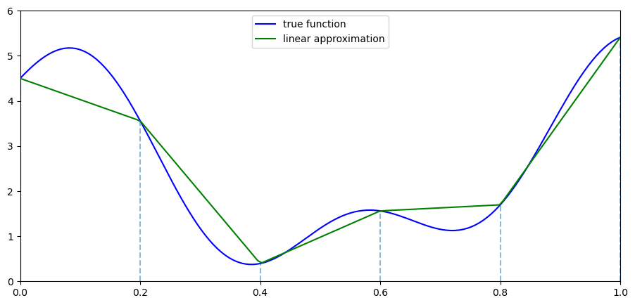
The next figure illustrates piecewise linear interpolation of an arbitrary function on grid points \(0, 0.2, 0.4, 0.6, 0.8, 1\).

def f(x):
    y1 = 2 * np.cos(6 * x) + np.sin(14 * x)
    return y1 + 2.5

c_grid = np.linspace(0, 1, 6)
f_grid = np.linspace(0, 1, 150)

def Af(x):
    return interp(c_grid, f(c_grid), x)

fig, ax = plt.subplots()

ax.plot(f_grid, f(f_grid), 'b-', label='true function')
ax.plot(f_grid, Af(f_grid), 'g-', label='linear approximation')
ax.vlines(c_grid, c_grid * 0, f(c_grid), linestyle='dashed', alpha=0.5)

ax.legend(loc="upper center")

ax.set(xlim=(0, 1), ylim=(0, 6))
plt.show()

_images/c9768bb76866e2d5a8aa4182a757c56326318a670460165e28d12878e9027e7f.png

16.3. Implementation #

The first step is to build a jitted class for the McCall model with separation and a continuous wage offer distribution.

We will take the utility function to be the log function for this application, with \(u(c) = \ln c\).

We will adopt the lognormal distribution for wages, with \(w = \exp(\mu + \sigma z)\) when \(z\) is standard normal and \(\mu, \sigma\) are parameters.

@njit
def lognormal_draws(n=1000, μ=2.5, σ=0.5, seed=1234):
    np.random.seed(seed)
    z = np.random.randn(n)
    w_draws = np.exp(μ + σ * z)
    return w_draws

Here’s our class.

mccall_data_continuous = [
    ('c', float64),          # unemployment compensation
    ('α', float64),          # job separation rate
    ('β', float64),          # discount factor
    ('w_grid', float64[:]),  # grid of points for fitted VFI
    ('w_draws', float64[:])  # draws of wages for Monte Carlo
]

@jitclass(mccall_data_continuous)
class McCallModelContinuous:

    def __init__(self,
                 c=1,
                 α=0.1,
                 β=0.96,
                 grid_min=1e-10,
                 grid_max=5,
                 grid_size=100,
                 w_draws=lognormal_draws()):

        self.c, self.α, self.β = c, α, β

        self.w_grid = np.linspace(grid_min, grid_max, grid_size)
        self.w_draws = w_draws

    def update(self, v, d):

        # Simplify names
        c, α, β = self.c, self.α, self.β
        w = self.w_grid
        u = lambda x: np.log(x)

        # Interpolate array represented value function
        vf = lambda x: interp(w, v, x)

        # Update d using Monte Carlo to evaluate integral
        d_new = np.mean(np.maximum(vf(self.w_draws), u(c) + β * d))

        # Update v
        v_new = u(w) + β * ((1 - α) * v + α * d)

        return v_new, d_new

We then return the current iterate as an approximate solution.

@njit
def solve_model(mcm, tol=1e-5, max_iter=2000):
    """
    Iterates to convergence on the Bellman equations

    * mcm is an instance of McCallModel
    """

    v = np.ones_like(mcm.w_grid)    # Initial guess of v
    d = 1                           # Initial guess of d
    i = 0
    error = tol + 1

    while error > tol and i < max_iter:
        v_new, d_new = mcm.update(v, d)
        error_1 = np.max(np.abs(v_new - v))
        error_2 = np.abs(d_new - d)
        error = max(error_1, error_2)
        v = v_new
        d = d_new
        i += 1

    return v, d

Here’s a function compute_reservation_wage that takes an instance of McCallModelContinuous and returns the associated reservation wage.

If \(v(w) < h\) for all \(w\), then the function returns np.inf

@njit
def compute_reservation_wage(mcm):
    """
    Computes the reservation wage of an instance of the McCall model
    by finding the smallest w such that v(w) >= h.

    If no such w exists, then w_bar is set to np.inf.
    """
    u = lambda x: np.log(x)

    v, d = solve_model(mcm)
    h = u(mcm.c) + mcm.β * d

    w_bar = np.inf
    for i, wage in enumerate(mcm.w_grid):
        if v[i] > h:
            w_bar = wage
            break

    return w_bar

The exercises ask you to explore the solution and how it changes with parameters.

16.4. Exercises #

Exercise 16.1

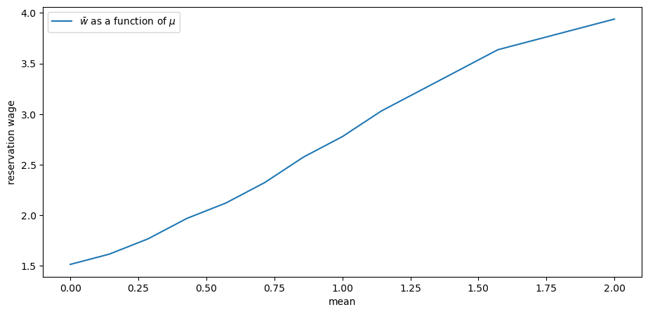
Use the code above to explore what happens to the reservation wage when the wage parameter \(\mu\) changes.

Use the default parameters and \(\mu\) in mu_vals = np.linspace(0.0, 2.0, 15).

Is the impact on the reservation wage as you expected?

Solution to Exercise 16.1

Here is one solution

mcm = McCallModelContinuous()
mu_vals = np.linspace(0.0, 2.0, 15)
w_bar_vals = np.empty_like(mu_vals)

fig, ax = plt.subplots()

for i, m in enumerate(mu_vals):
    mcm.w_draws = lognormal_draws(μ=m)
    w_bar = compute_reservation_wage(mcm)
    w_bar_vals[i] = w_bar

ax.set(xlabel='mean', ylabel='reservation wage')
ax.plot(mu_vals, w_bar_vals, label=r'$\bar w$ as a function of $\mu$')
ax.legend()

plt.show()

_images/8daa26f8b264a9c48ff53c9b179ce5a3b1f10b7a0b3d185c6ebf4f0ca5f4df5d.png

Not surprisingly, the agent is more inclined to wait when the distribution of offers shifts to the right.

Exercise 16.2

Let us now consider how the agent responds to an increase in volatility.

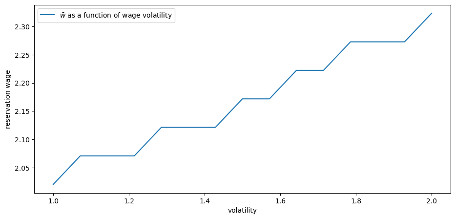
To try to understand this, compute the reservation wage when the wage offer distribution is uniform on \((m - s, m + s)\) and \(s\) varies.

The idea here is that we are holding the mean constant and spreading the support.

(This is a form of mean-preserving spread.)

Use s_vals = np.linspace(1.0, 2.0, 15) and m = 2.0.

State how you expect the reservation wage to vary with \(s\).

Now compute it. Is this as you expected?

Solution to Exercise 16.2

Here is one solution

mcm = McCallModelContinuous()
s_vals = np.linspace(1.0, 2.0, 15)
m = 2.0
w_bar_vals = np.empty_like(s_vals)

fig, ax = plt.subplots()

for i, s in enumerate(s_vals):
    a, b = m - s, m + s
    mcm.w_draws = np.random.uniform(low=a, high=b, size=10_000)
    w_bar = compute_reservation_wage(mcm)
    w_bar_vals[i] = w_bar

ax.set(xlabel='volatility', ylabel='reservation wage')
ax.plot(s_vals, w_bar_vals, label=r'$\bar w$ as a function of wage volatility')
ax.legend()

plt.show()

_images/960ce6be53aada090ecead7657246708d446d69c37f3254befcf13475e1dc0c3.png

The reservation wage increases with volatility.

One might think that higher volatility would make the agent more inclined to take a given offer, since doing so represents certainty and waiting represents risk.

But job search is like holding an option: the worker is only exposed to upside risk (since, in a free market, no one can force them to take a bad offer).

More volatility means higher upside potential, which encourages the agent to wait.

16. Job Search III: Fitted Value Function Iteration#

16.1. Overview#

16.2. The Algorithm#